The chief purpose of an endowment’s spending policy is to manage the tension between current and future needs. How much of your endowment should be used for immediate needs? And what portion should be invested for the future? Setting the right spending policy is critical for a school’s long-term viability. However, most schools use a methodology which threatens their ability to provide consistent funding. Schools must consider whether their spending policy is aligned with their spending needs and select a methodology that maintains stable spending throughout market cycles. This will enable your school to fulfill its missions irrespective of market movements.
Moving Average Methodology: Pros and Cons
Most independent schools (and most nonprofits) employ the Moving Average methodology to calculate their endowment spending rate. This methodology bases spending on the average market value of the endowment over a specified time period (typically the past 3 years or trailing 12 quarters).
Annual Spend = Average 3-Year Endowment Market Value * Spending Rate (%)
Using this methodology, spending will vary based on investment returns. It serves as a handbrake to reduce spending when the markets perform poorly and to increase spending after the markets have had strong returns. The perceived benefit to this approach is that in times of market stress, reduced spending can in part compensate for poor market returns and preserve the endowment for future spending needs. However, this runs contrary to a school’s needs. In tough economic times, schools require more stable funding from the endowment to meet day-to-day operating expenses.
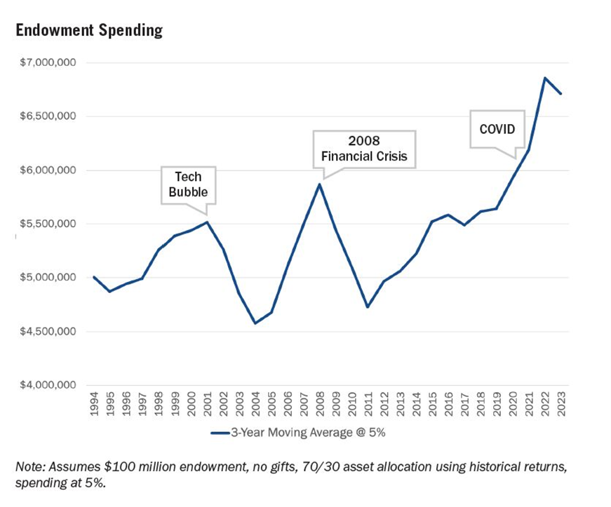
With endowment spending levels tied to market value, the Moving Average methodology results in significant spending volatility, making it hard for schools to appropriately budget for staffing, programs and other operating needs. The chart below illustrates this effect on a hypothetical $100 million school endowment. Over the past 30 years, the school’s annual endowment spend would have fluctuated between a low of $4.5 million and a high of $6.8 million. Spending would have declined by $935,000 following the tech bubble in 2001 and $1.1 million following the 2008 financial crisis. After the financial crisis, it would have taken 10 years for spending to recover to 2008 levels.
Constant Growth Methodology: Pros and Cons
To minimize spending volatility and enhance revenue diversification, we advise our independent school clients to utilize the Constant Growth spending methodology. While only 2% of schools currently use this approach, we believe it is the most congruent with their needs. Endowment spending grows each year at a predetermined rate of inflation and expectations for gift flow.
Annual Spend = Current Endowment Spend * [Inflation Rate(%) + Gift Growth Rate(%)]
While there are many factors to consider when choosing the inflation rate, organizations typically use the Consumer Price Index (CPI), the Higher Education Price Index (HEPI) or a rate that is more in line with the annual increase in their operating budget.
Unlike the Percentage of Moving Average method, the Constant Growth model separates spending from normal market volatility. As a result, spending rates can be higher in times of poor market performance, when net tuition rates and gifts are under pressure, and lower in strong markets, when savings can be reinvested in the endowment and compound at a higher rate of return. The Constant Growth model also enables schools to better control spending through adjustments in the inflation factor. By lowering the inflation rate, schools can slowly reduce their spending rate over time and minimize the disruption to operations.
To prevent a disconnect between endowment spending and market value, floors and caps are often used to set an acceptable spending range. For example, a 5.5% cap means spending will not exceed 5.5% of the endowment’s market value. Similarly, a 3% floor means spending will not be less than 3% of the endowment’s market value.
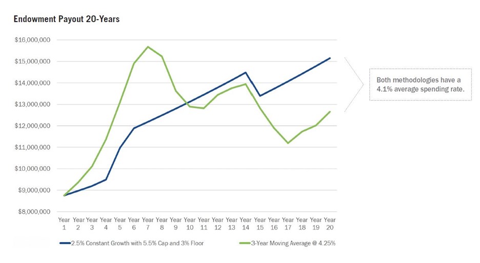
The chart above compares the spending volatility of the Constant Growth method (blue line) to the Percentage of Moving Average method (green line). Over this time frame, the Percentage of Moving Average model is much more volatile than the Constant Growth model–yet both methodologies have the same average spending rate of 4.1%. The Constant Growth methodology makes annual spending more predictable, smooths revenues and thus facilitates more consistent budgeting.
The most common criticism of the Constant Growth methodology is its failure to account for market value fluctuations. If the capital markets have a challenging year, the Constant Growth model allows for the previous year’s spending in dollars plus the rate of inflation to be spent. Likewise, in an environment of strong investment returns, the Constant Growth model will call for spending less than the Moving Average model would.
This criticism is actually the strength of the model. Schools often need to spend more in times of crisis and less in good economic times. Net tuition rates and annual gifts can be impacted significantly by the market cycle, making the annual endowment draw a critical source of revenue for the school. While the Constant Growth methodology is not widely used by independent schools, many of the highly endowment-dependent colleges and universities use it to calculate their spending levels.
The Hybrid Method: A Hybrid Approach
Some schools use a blend of the Constant Growth and Moving Average models to address the need for more market impact on endowment spending. This is referred to as the "Hybrid" methodology and used by 9% of all schools.
The Hybrid methodology leads to relatively smooth spending which has more volatility than the Constant Growth methodology, but significantly less volatility than the Moving Average methodology. The downside of the Hybrid is model is that it is more complex to implement than the other models.
Annual Spend = (60% to 80%) * Constant Growth + (20% to 40%) * Moving Average
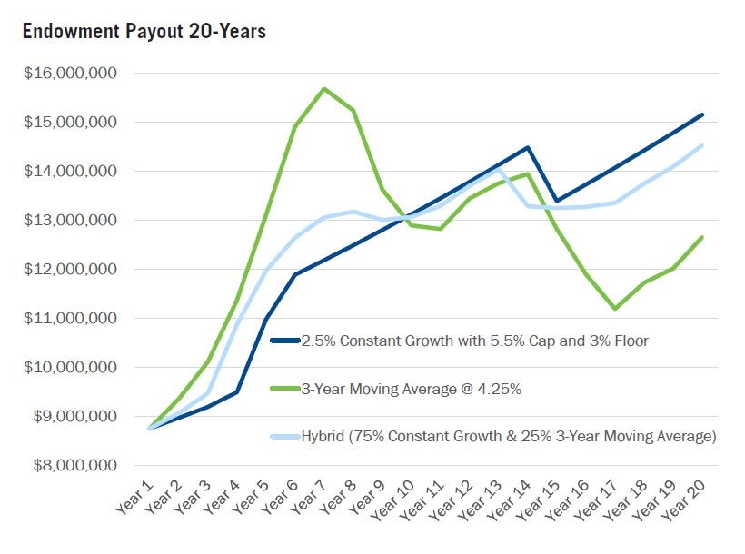
In the chart to above, the Hybrid model (light blue line) has a slightly more volatile path than the Constant Growth model (dark blue line), but both of these are much less volatile than the 3-year Moving Average (the green line.) In 20 years, a school would have the smoothest spending path if it used the Constant Growth methodology, but the Hybrid methodology also reduces the volatility significantly.
A Spending Policy You Can Maintain
The Constant Growth methodology is easier to sustain year over year because spending will not decrease, which limits the probability that you will seek additional endowment funds to shore up operations. However, with the Moving Average approach, in a dramatic financial downturn, you may be required to cut spending by 15%. In this situation, institutions are far more likely to disregard the spending formula and increase spending outright. And overspending has disastrous long-term ramifications.
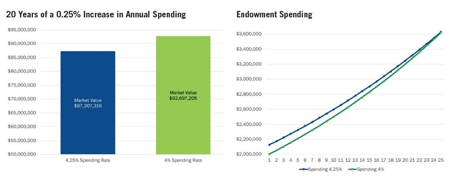
Increasing spending on a $50 million endowment by $125,000 (from 4% to 4.5%) may seem like the easiest way to solve a small operating deficit. Indeed, over 25 years, a 4.25% spending rate produces incremental spending. However, there is a cost associated with that spending. Due to the lower spending, the 4% payout model compounds to reach a market value of $92.7 million in 25 years, which is $5.5 million higher than the market value of the 4.25% model. This, in turn, allows the spending from the 4% model to be higher.
Over 25 years, the effect of compounding is so powerful that the portfolio with a 4% spending rate has a greater endowment payout than the portfolio with a 4.25% spending rate. This is demonstrated in the righthand chart below — by year 25, the spending at 4% (green line) outpaces the spending at 4.25% (blue line.)
Choosing a spending methodology that meets your objectives is critical for your school’s long-term health. It is critical that your endowment manager engage in extensive financial modeling and analysis to create a spending policy to meet your school’s unique needs.